Using Firefly to Explore OpenUniverse2024 Simulated Roman and Rubin Images

Learning Goals¶

By the end of this tutorial, you will:

• Learn how to access cloud-hosted Roman and Rubin simulated images.

• Learn how to find the Roman and Rubin images covering a sky position with the IRSA Simple Image Access (SIA) service.

• Learn how to launch an interactive Firefly instance inside JupyterLab.

• Learn how to use the Firefly Jupyterlab extension to visualize cloud-hosted simulated images, overplot ds9 regions, overplot catalogs in Parquet format, and create 3 color images.

Introduction¶

The purpose of this tutorial is to become familiar with the simulated Roman and Rubin data published through OpenUniverse2024, and to become familiar with the Firefly JupyterLab Extension for visualizing astronomical data products.

OpenUniverse2024 is a project to simulate spatially overlapping imaging surveys to be carried out by the Nancy Grace Roman Telescope and the Vera C. Rubin Observatory. The simulations were carried out on Argonne’s Theta cluster and consist of:

• The LSST ELAIS-S1 Deep Drilling Field (DDF)

• The Roman Time-Domain Survey (TDS) shifted to overlap the ELAIS region and LSST DDF

• Overlapping LSST Wide-Fast-Deep (WFD) survey (with rolling cadence)

• Overlapping Roman Wide-Area Survey (WAS) in the same region

• A deep-field calibration region of the Roman WAS in the same region

This tutorial works with the full simulation, which covers the entire survey footprint. More information about the dataset can be found at IRSA’s holding of this dataset, and the OpenUniverse2024 paper describes how the simulation was produced.

Firefly is an open-source web-based UI library for astronomical data archive access and visualization developed at Caltech and used by multiple space- and ground-based astrophysics archives. More information on Firefly can be found here.

In addition to being used to make web applications, Firefly can be used from Python. More information on Firefly Python client can be found here.

The Firefly JupyterLab Extension makes it particularly easy to use Firefly to efficiently visualize cloud-hosted astronomical data using JupyterLab instances running locally or on cloud. More information on Firefly JupyterLab Extension can be found here.

If you are new to OpenUniverse2024, the Quickstart tutorial introduces the directory layout, the parquet catalogs, and the SIA image search that this notebook builds on.

Imports¶

• astropy.io.fits for accessing FITS files

• numpy for numerical computing

• matplotlib.pyplot for creating static visualizations of FITS images

• matplotlib.patches for annotating visualizations of FITS images

• astropy.wcs for dealing with astronomical world coordinate systems

• astropy.units for dealing with astronomical units

• astropy.coordinates.SkyCoord for dealing with astronomical coordinates

• astroquery.ipac.irsa.Irsa for asking IRSA which images cover a position

• hpgeom for converting a sky position into a HEALPix region index

• json for reading the cloud location returned by the image search

• firefly_client.FireflyClient for using the Firefly python client

• astropy.nddata.Cutout2D for making image cutouts

• reproject.reproject_interp for rotating cutouts so both telescopes’ panels point the same way

• io.BytesIO for writing a fits file to an in-memory stream

# Uncomment the next line to install dependencies if needed.
# !pip install numpy astropy s3fs matplotlib firefly_client astroquery hpgeom reproject

from astropy.io import fits
import numpy as np
from matplotlib import pyplot as plt
from matplotlib import patches
from astropy import wcs
from astropy import units as u
from astropy.coordinates import SkyCoord
from astroquery.ipac.irsa import Irsa
import hpgeom
import json
from firefly_client import FireflyClient
from astropy.nddata import Cutout2D
from reproject import reproject_interp
from io import BytesIO

1. Learn where the OpenUniverse2024 data are hosted in the cloud¶

The OpenUniverse2024 data are hosted in the cloud via Amazon Web Services (AWS). To access these data, you need to create a client to read data from Amazon’s Simple Storage Service (s3) buckets, and you need to know some information about those buckets. OpenUniverse2024 contains simulations of the Roman Wide-Area Survey (WAS) and the Roman Time Domain Survey (TDS). In this tutorial, we will focus on the WAS.

We ask IRSA’s Simple Image Access (SIA) service to locate both the Roman and Rubin images by coordinate.

BUCKET_NAME = "nasa-irsa-simulations"
OU_PREFIX = "openuniverse2024"
TRUTH_FILES_PATH = f"{OU_PREFIX}/roman/full/roman_rubin_cats_v1.1.2_faint"

# Point the astroquery IRSA client at the simulated-data services, which are
# separate from the ones serving IRSA's observed data.
Irsa.sia_url = "https://irsa.ipac.caltech.edu/simulated/SIA"
Irsa.tap_url = "https://irsa.ipac.caltech.edu/simulated/TAP"

OU_ROMAN_SIA_COLLECTION = "simulated_roman_openuniverse2024"
OU_RUBIN_SIA_COLLECTION = "simulated_rubin_openuniverse2024"

# A small radius is all we need, since we only want images containing a given point.
SEARCH_RADIUS = 1 * u.arcsec

2. Roman Images¶

The Nancy Grace Roman Space Telescope will carry out a wide-area survey (WAS) in the near infrared. OpenUniverse2024 simulates that survey as individual exposures, each covering one detector’s worth of sky. Bands include F184, H158, J129, K213, W146, Y106.

The survey stores those exposures by pointing and detector rather than by sky position, so in this section we define a function that asks the image search which exposure covers a position, and then reads it.

Define a function that retrieves a Roman simulated image given a sky position and filter.¶

The Roman collection holds both the Wide-Area Survey and the Time Domain Survey, so we keep only the WAS exposures and then only the band we want. Many exposures cover any given position, so we sort by observation time and take the earliest.

Having found the file, we prefix its path with s3:// and open it with astropy. The science image sits in the first extension, and we take the WCS from the same header as an astropy.wcs.WCS object. The function returns a dictionary of both, along with the header itself so we can look at it later, and the path so that later cells can reuse it instead of searching a second time.

def get_roman_image(coord, filter):
    """Read the Roman WAS exposure covering a position in a given filter.

    Parameters
    ----------
    coord : `~astropy.coordinates.SkyCoord`
        Sky position to search around.
    filter : str
        Roman bandpass name, e.g. ``'H158'``.

    Returns
    -------
    dict
        Keys ``'data'`` (`~numpy.ndarray`), ``'wcs'`` (`~astropy.wcs.WCS`),
        ``'header'`` (`~astropy.io.fits.Header`) and ``'fpath'`` (str, the S3
        path of the exposure).

    Raises
    ------
    ValueError
        If no WAS exposure in that filter covers ``coord``.
    """
    results = Irsa.query_sia(pos=(coord, SEARCH_RADIUS),
                             collection=OU_ROMAN_SIA_COLLECTION)

    in_was = results[['WAS_simple_model' in str(r['obs_id']) for r in results]]
    in_band = in_was[[str(r['energy_bandpassname']).strip() == filter
                      for r in in_was]]
    if len(in_band) == 0:
        raise ValueError(f"No Roman WAS {filter}-band images cover "
                         f"{coord.to_string('hmsdms')}")

    in_band.sort('t_min')
    cloud_info = json.loads(in_band['cloud_access'][0])['aws']
    image_s3_fpath = f"{cloud_info['bucket_name']}/{cloud_info['key']}"

    with fits.open(f"s3://{image_s3_fpath}", fsspec_kwargs={"anon": True}) as hdul:
        # retrieve science data, which sits in the first extension
        image_data = hdul[1].data

        # make wcs using header
        image_wcs = wcs.WCS(hdul[1].header)

        return {'data': image_data, 'wcs': image_wcs, 'header': hdul[1].header,
                'fpath': image_s3_fpath}

Inspect a simulated Roman image¶

Choose a filter and a position within the survey footprint

coord = SkyCoord(ra=9.6205000, dec=-44.0641694, unit="deg")
filter_roman = 'H158' #F184, H158, J129, K213, W146, and Y106 are available

Retrieve the data and header information from the simulated Roman image corresponding to the chosen position and filter.

image_roman = get_roman_image(coord, filter_roman)

WARNING: FITSFixedWarning: 'datfix' made the change 'Changed DATE-OBS from '2028-05-19 13:41:34.224000' to '2028-05-19T13:41:34.224000''. [astropy.wcs.wcs]

Understand the size of a simulated Roman image.¶

# Number of pixels (Y, X)
image_roman['data'].shape

# Pixel size (scale Y, scale X) [degrees/pixel]
image_roman['wcs'].proj_plane_pixel_scales()

# Image size (FOV Y, FOV X)
[(num * size).to('arcsec') for num, size in zip(
    image_roman['data'].shape, image_roman['wcs'].proj_plane_pixel_scales())]

The field of view of a Roman exposure is ~450 arcsec, at a pixel scale of ~0.11 arcsec.

Look at everything else the image file contains¶

So far we have read the science image, but each exposure carries more than that. Listing the extensions shows the full picture.

with fits.open(f"s3://{image_roman['fpath']}",
               fsspec_kwargs={"anon": True}) as hdul:
    hdul.info()

Filename: <class 's3fs.core.S3File'>
No.    Name      Ver    Type      Cards   Dimensions   Format
  0  PRIMARY       1 PrimaryHDU      63   ()      
  1  SCI           1 ImageHDU        68   (4088, 4088)   float64   
  2  ERR           1 ImageHDU        68   (4088, 4088)   float32   
  3  DQ            1 ImageHDU        70   (4088, 4088)   int32 (rescales to uint32)   

Each file holds a primary header carrying the observation metadata but no pixels, followed by three 4088x4088 planes:

SCI = the simulated science image, in electrons per second

ERR = the estimated uncertainty on each science pixel

DQ = the data quality mask, flagging pixels that should not be trusted

Use the WCS from the Roman simulated header to convert the specified coordinate into a pixel position.¶

def coord_to_xy(w, coord):
    """Convert a sky position into (x, y) pixel indices.

    Parameters
    ----------
    w : `~astropy.wcs.WCS`
        WCS of the image the indices refer to.
    coord : `~astropy.coordinates.SkyCoord`
        Sky position to convert.

    Returns
    -------
    tuple of int
        Pixel indices as ``(x, y)``.
    """
    return w.world_to_array_index(coord)[::-1] #reverse since 0th axis is y, 1st axis is x

coord_arr_idx = coord_to_xy(image_roman['wcs'], coord)
coord_arr_idx

Use matplotlib imshow to create a static visualization of the Roman simulated image and overplot the selected position.¶

Each telescope points independently, so neither survey’s images arrive with north pointing up: this Roman exposure is turned about 170 degrees from north, and the Rubin visit in the next section about 160 degrees. Every figure in this notebook is therefore resampled onto a north-up grid before plotting, so that all of them, and both telescopes, can be read the same way. The rotation leaves the frame tilted inside a slightly larger box, with empty wedges in the corners.

def stretch_color(data, clipPercent):
    """Percentile clip limits for displaying an image.

    Parameters
    ----------
    data : `~numpy.ndarray`
        Image values; NaNs are ignored.
    clipPercent : float
        Percentage clipped off each end of the distribution.

    Returns
    -------
    tuple of float
        Lower and upper limits, for passing to ``clim``.
    """
    # nan-aware: rotating to north up leaves empty corners
    return np.nanpercentile(data, (0 + clipPercent, 100 - clipPercent))


def north_up(data, image_wcs, size, binning=1):
    """Resample onto a north-up grid, keeping the original pixel scale.

    Parameters
    ----------
    data : `~numpy.ndarray`
        Image to resample.
    image_wcs : `~astropy.wcs.WCS`
        WCS of ``data``.
    size : `~astropy.units.Quantity`
        Angular width of the output grid.
    binning : int, optional
        Sample this many input pixels per output pixel. Values greater than 1
        are enough for displaying a whole exposure and much quicker than
        resampling every pixel.

    Returns
    -------
    `~numpy.ndarray`
        The resampled image.
    `~astropy.wcs.WCS`
        WCS of the resampled image.
    """
    scale = abs(image_wcs.proj_plane_pixel_scales()[0].to(u.deg).value) * binning
    npix = int(round(size.to(u.deg).value / scale))

    ny, nx = data.shape
    center = image_wcs.pixel_to_world((nx - 1) / 2, (ny - 1) / 2)

    target = wcs.WCS(naxis=2)
    target.wcs.ctype = ['RA---TAN', 'DEC--TAN']
    target.wcs.crpix = [(npix + 1) / 2, (npix + 1) / 2]
    target.wcs.crval = [center.ra.deg, center.dec.deg]
    target.wcs.cdelt = [-scale, scale]

    return reproject_interp((data, image_wcs), target, shape_out=(npix, npix))[0], target


def full_frame_north_up(image, binning=4):
    """North-up view of a whole exposure, for display only.

    Parameters
    ----------
    image : dict
        Image dictionary with ``'data'`` and ``'wcs'`` keys, as returned by
        `get_roman_image` or `get_rubin_image`.
    binning : int, optional
        Sample this many input pixels per output pixel.

    Returns
    -------
    `~numpy.ndarray`
        The resampled image.
    `~astropy.wcs.WCS`
        WCS of the resampled image.
    """
    ny, nx = image['data'].shape
    fov = nx * image['wcs'].proj_plane_pixel_scales()[0].to(u.arcsec)
    return north_up(image['data'], image['wcs'], 1.2 * fov, binning=binning)

roman_display, roman_display_wcs = full_frame_north_up(image_roman)

plt.imshow(roman_display, origin='lower', 
           clim=stretch_color(roman_display, 1)
           )

plt.plot(*coord_to_xy(roman_display_wcs, coord), 'o', mfc='none', mec='r',
         markersize=15, markeredgewidth=2)
plt.axis('off')

(np.float64(-0.5), np.float64(1225.5), np.float64(-0.5), np.float64(1225.5))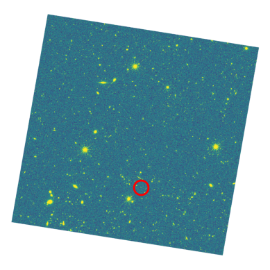

3. Rubin Images¶

OpenUniverse2024 includes simulated Rubin images in the following filters: u, g, r, i, z, y. As with Roman, these are stored by visit and detector rather than by sky position, so we again let the SIA service tell us which images cover our position. In this section, we define functions that retrieve a Rubin image for a chosen position and filter, returning data in the same structure as the function we defined above for Roman.

Retrieve Rubin images¶

The image search returns one row per image, with the cloud location of each tucked inside a cloud_access JSON string. Many visits cover any given position, so we sort by observation time and take the earliest.

def get_rubin_image_fpaths(coord, filters):
    """Find the Rubin images covering a position in each of several filters.

    Parameters
    ----------
    coord : `~astropy.coordinates.SkyCoord`
        Sky position to search around.
    filters : list of str
        Rubin bandpass names, e.g. ``['g', 'r', 'i']``.

    Returns
    -------
    dict
        Filter name to S3 path of the image covering ``coord``.

    Raises
    ------
    ValueError
        If any requested filter has no image covering ``coord``.
    """
    # One search covers every band, so ask once and sort the results out by band
    # afterwards rather than searching again for each one.
    results = Irsa.query_sia(pos=(coord, SEARCH_RADIUS),
                             collection=OU_RUBIN_SIA_COLLECTION)

    fpaths = {}
    for filter in filters:
        # Band names come back like "r_57", so compare only the part before the underscore.
        in_band = results[[str(r['energy_bandpassname']).split('_')[0] == filter
                           for r in results]]
        if len(in_band) == 0:
            raise ValueError(f"No Rubin {filter}-band images cover "
                             f"{coord.to_string('hmsdms')}")

        in_band.sort('t_min')
        cloud_info = json.loads(in_band['cloud_access'][0])['aws']
        fpaths[filter] = f"{cloud_info['bucket_name']}/{cloud_info['key']}"

    return fpaths

def get_rubin_image(coord, filter):
    """Read the Rubin image covering a position in a given filter.

    Parameters
    ----------
    coord : `~astropy.coordinates.SkyCoord`
        Sky position to search around.
    filter : str
        Rubin bandpass name, e.g. ``'r'``.

    Returns
    -------
    dict
        Keys ``'data'`` (`~numpy.ndarray`), ``'wcs'`` (`~astropy.wcs.WCS`) and
        ``'fpath'`` (str, the S3 path of the image).
    """
    image_s3_fpath = get_rubin_image_fpaths(coord, [filter])[filter]

    with fits.open(f"s3://{image_s3_fpath}", fsspec_kwargs={"anon": True}) as hdul:
        # retrieve science data, which sits in the first extension
        image_data = hdul[1].data

        # make wcs using header
        image_wcs = wcs.WCS(hdul[1].header)

        # hand back the path too, so later cells can reuse it instead of
        # asking the image search for it a second time
        return {'data': image_data, 'wcs': image_wcs, 'fpath': image_s3_fpath}

Inspect a simulated Rubin image¶

Choose a filter and retrieve the data and header information from the simulated Rubin image covering our position.

filter_rubin = 'r'
image_rubin = get_rubin_image(coord, filter_rubin)

Understand the size of a simulated Rubin image.¶

# Number of pixels (Y, X)
image_rubin['data'].shape

# Pixel size (scale Y, scale X) [degrees/pixel]
image_rubin['wcs'].proj_plane_pixel_scales()

# Image size (FOV Y, FOV X)
[(num * size).to('arcsec') for num, size in zip(
    image_rubin['data'].shape, image_rubin['wcs'].proj_plane_pixel_scales())]

A single Rubin detector covers a somewhat larger patch of sky than one Roman exposure, at roughly twice the pixel scale.

Use matplotlib imshow to create a static visualization of the Rubin simulated image and overplot the selected position.¶

The two full-frame figures do not cover the same patch of sky. Each is centered on its own exposure and sized to its own field of view, so the Rubin panel is nearly twice as wide on the sky as the Roman one. What they share is the marked position, which falls inside both.

rubin_display, rubin_display_wcs = full_frame_north_up(image_rubin)

plt.imshow(rubin_display, origin='lower', 
           clim=stretch_color(rubin_display, 1)
           )

plt.plot(*coord_to_xy(rubin_display_wcs, coord), 'o', mfc='none', mec='r',
         markersize=15, markeredgewidth=2)
plt.axis('off')

(np.float64(-0.5), np.float64(1228.5), np.float64(-0.5), np.float64(1228.5))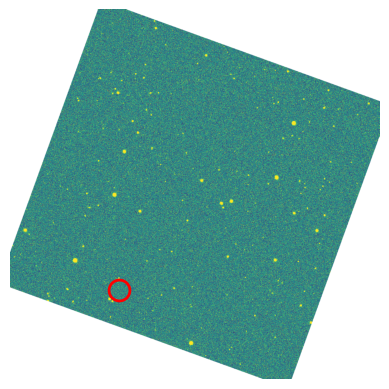

4. Compare simulated Roman and Rubin cutouts for a selected position¶

Choose cutout size¶

cutout_size = 50*u.arcsec

Create the cutouts¶

# Cut oversized: the rotation below needs data in the corners to draw from.
cutout_roman = Cutout2D(image_roman['data'], coord, size=1.5*cutout_size, wcs=image_roman['wcs'])
cutout_rubin = Cutout2D(image_rubin['data'], coord, size=1.5*cutout_size, wcs=image_rubin['wcs'])

Rotate both cutouts so that north points up¶

The full frames above were rotated for display; here we do the same to the cutouts, using the same helper. The two telescopes are turned about 10 degrees apart from each other, so without this the panels would not line up. Each keeps its own pixel scale, so Roman still shows the finer sampling.

# Rotating a same-size grid would leave empty corners, so each cutout above was cut
# oversized and is resampled down to the size we actually want.
roman_data, roman_wcs = north_up(cutout_roman.data, cutout_roman.wcs, cutout_size)
rubin_data, rubin_wcs = north_up(cutout_rubin.data, cutout_rubin.wcs, cutout_size)

Use matplotlib imshow to plot static side-by-side comparisons of the cutouts¶

fig, axs = plt.subplots(1, 2, figsize=(12, 6))


axs[0].imshow(roman_data, origin='lower', 
              clim=stretch_color(roman_data, .5)
              )
axs[0].set_title(f"ROMAN in filter {filter_roman}")

axs[1].imshow(rubin_data, origin='lower', 
              clim=stretch_color(rubin_data, .5)
              )
axs[1].set_title(f"RUBIN in filter {filter_rubin}")

fig.suptitle(f"Cutouts at ({coord.ra}, {coord.dec}) with {cutout_size} size", fontsize=14)
plt.tight_layout(rect=[0, 0, 1, 0.97])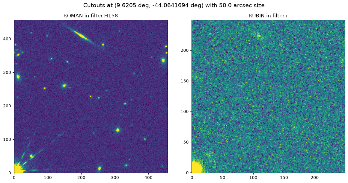

Both panels cover the same patch of sky, at the same size and with north up in each. The difference is stark: the simulated Roman exposure resolves a field full of galaxies, while the same patch in the simulated Rubin image is close to blank. A single Rubin visit is short, so only the brightest sources here rise above its noise, and from the ground its point spread function is broad enough to blend close neighbors together. Roman’s finer pixels and sharper point spread function keep those sources separate. Rubin reaches its full depth by stacking many visits, which is not what we are looking at.

5. Use Firefly to interactively explore the images¶

Static cutouts only help once you know where to look. Choosing a position worth comparing means exploring the image interactively, and for that we hand it to Firefly. In this section we display the simulated Rubin visit, outline the area the Roman exposure covers, and pan and zoom around it to pick out a target.

Launch and initialize Firefly¶

There are two ways to initialize a Firefly client from Python, depending on whether you’re running the notebook in JupyterLab or not. Assuming you have jupyter-firefly-extensions set up in your environment as explained here, you can use make_lab_client() in JupyterLab, which will open the Firefly viewer in a new tab within the Lab. Otherwise, you can use make_client() in a Jupyter Notebook (or even a Python shell), which will open the Firefly viewer in a new web browser tab.

You also need a Firefly server to communicate with your Firefly Python client. In this notebook, we use a public Firefly server: the IRSA Viewer (https://irsa.ipac.caltech.edu/irsaviewer). However, you can also run a local Firefly server via a Firefly Docker image and access it at http://localhost:8080/firefly. The URL of the Firefly server is read by both make_client() and make_lab_client() through the environment variable FIREFLY_URL. However, make_client() also allows you to pass the URL directly as the url parameter.

# Uncomment when using within Jupyter Lab with jupyter_firefly_extensions installed
# fc = FireflyClient.make_lab_client()

# Uncomment for contexts other than above 
fc = FireflyClient.make_client(url="https://irsa.ipac.caltech.edu/irsaviewer")

fc.reinit_viewer() # to clean the state, if this cell ran earlier

Define a function that returns the URL for a given S3 filepath¶

Since the OpenUniverse2024 data are in a public S3 bucket, any file can also be reached over HTTPS. Firefly loads images and catalogs by URL rather than by S3 path, so we use this helper throughout the rest of the notebook.

def https_url(s3_fpath):
    """Convert an S3 path into a public HTTPS URL.

    Parameters
    ----------
    s3_fpath : str
        Path of the form ``'bucket/key'``.

    Returns
    -------
    str
        HTTPS URL for the same file.
    """
    s3_fpath_without_bucket = s3_fpath.split('/', 1)[1]
    return f"https://{BUCKET_NAME}.s3.amazonaws.com/{s3_fpath_without_bucket}"

Let’s generate URL for the Rubin image we plotted above. Clicking on the returned URL will allow you to download this image locally.

image_s3_fpath_rubin = image_rubin['fpath']
https_url(image_s3_fpath_rubin)

Send the simulated Rubin image to Firefly using show_fits.¶

For displaying the FITS image of the Rubin visit in Firefly, we use show_fits:

image_ff_id_rubin = 'rubin-image-filter-r'
fc.show_fits(url=https_url(image_s3_fpath_rubin),
             plot_id=image_ff_id_rubin,
             Title="Rubin Image"
             )

WARNING: show_fits() is deprecated. Use show_fits_image() instead.
WARNING: url is deprecated, use file_input parameter instead

Use ds9 region syntax to outline the Roman exposure on the interactive display¶

The Firefly client includes several methods related to controlling ds9 region overlays. To overlay a region layer on the loaded FITS images, we can use overlay_region_layer.

Region data is defined in ds9 region syntax that can be found here.

The Rubin visit on display covers more sky than the Roman exposure does, so it is worth seeing where the Roman data actually falls. The corners of the Roman exposure come straight from its WCS, and we draw them as a polygon.

roman_corners = image_roman['wcs'].calc_footprint()
roman_corners

# outline the Roman exposure as a polygon
corner_coords = ' '.join(f'{ra}d {dec}d' for ra, dec in roman_corners)
roman_regions = [f'icrs;polygon {corner_coords} # text={{Roman {filter_roman}}}']

roman_regions_id = 'roman_regions'
# Name the plot explicitly. Without plot_id the layer goes to whichever plot is
# active, which is not necessarily this one if cells are run out of order.
fc.overlay_region_layer(region_data=roman_regions,
                        title='Roman exposure', 
                        region_layer_id=roman_regions_id,
                        plot_id=image_ff_id_rubin)

Use Firefly’s pan and zoom capabilities to locate a region of interest¶

You can view the coordinates of your mouse pointer at the bottom left of the display window. To copy the coordinates for a specific coordinate:

• Toggle the “Click Lock” to “on” in the bottom right of the image display.

• Click on the position of interest, and notice that the coordinate display is now frozen.

• Click on “EQ-J2000”, the coordinate label in the bottom left of the image display. The pop-up that opens lets you choose the coordinate system, and the format used when copying — pick the Python format so the value can be pasted straight into a SkyCoord.

• Close the pop-up and click the small clipboard icon next to the coordinate readout.

Copy the coordinates from the coordinate display to the Python notebook¶

The position we have been using since Section 2 is the one marked below, so by default we carry it forward. Paste a position of your own here instead to compare a different target.

coords_of_interest = coord  # or e.g. SkyCoord('0h38m28.92s -44d03m51.01s', frame='icrs')
coords_of_interest

We can now use this astropy SkyCoord object to compare our images.

Use ds9 region syntax to overplot the selected position¶

For this we use the id of the region layer we defined above, and add more region data using add_region_data.

point_region = f'icrs;point {coords_of_interest.ra.value}d {coords_of_interest.dec.value}d # point=cross 15 text={{Source of interest}}'
fc.add_region_data(region_data=point_region, region_layer_id=roman_regions_id,
                   plot_id=image_ff_id_rubin)

6. Plot cutouts of the identified source¶

This is a small group of galaxies, with a close neighbour 2.7 arcsec away. Roman shows them as separate objects; in Rubin they sit at the level of the noise. The Rubin image is a single visit rather than a stack, so faint sources like these are simply not detected in it, which is worth keeping in mind when comparing the two panels below.

# The images from Sections 2 and 3 already cover the default position, so only
# re-read if you pasted a different one above.
if coords_of_interest.separation(coord) > 0*u.arcsec:
    image_roman = get_roman_image(coords_of_interest, filter_roman)
    image_rubin = get_rubin_image(coords_of_interest, filter_rubin)

cutout_size = 8*u.arcsec

# As in section 4, cut oversized and then rotate both to north up.
cutout_roman = Cutout2D(image_roman['data'], coords_of_interest, size=1.5*cutout_size, wcs=image_roman['wcs'])
cutout_rubin = Cutout2D(image_rubin['data'], coords_of_interest, size=1.5*cutout_size, wcs=image_rubin['wcs'])

roman_data, roman_wcs = north_up(cutout_roman.data, cutout_roman.wcs, cutout_size)
rubin_data, rubin_wcs = north_up(cutout_rubin.data, cutout_rubin.wcs, cutout_size)

fig, axs = plt.subplots(1, 2, figsize=(12, 6))

axs[0].imshow(roman_data, origin='lower', 
              clim=stretch_color(roman_data, .5)
              )
axs[0].set_title(f"ROMAN in filter {filter_roman}")

# Let's also encircle the source we identified. The circle is 2 arcsec across
# on both panels, so the two cutouts can be compared directly despite their different
# pixel scales.
roman_scale = roman_wcs.proj_plane_pixel_scales()[0].to(u.arcsec).value
axs[0].add_patch(patches.Circle(coord_to_xy(roman_wcs, coords_of_interest), 
                                radius=2/roman_scale, color='r', fill=False, linewidth=2))


axs[1].imshow(rubin_data, origin='lower', 
              clim=stretch_color(rubin_data, .5)
              )
axs[1].set_title(f"RUBIN in filter {filter_rubin}")

# Let's also encircle the source we identified 
rubin_scale = rubin_wcs.proj_plane_pixel_scales()[0].to(u.arcsec).value
axs[1].add_patch(patches.Circle(coord_to_xy(rubin_wcs, coords_of_interest),
                                radius=2/rubin_scale, color='r', fill=False, linewidth=2))


fig.suptitle(f"Cutouts at ({coords_of_interest.ra:6f}, {coords_of_interest.dec:6f}) with {cutout_size} size", fontsize=14);
plt.tight_layout(rect=[0, 0, 1, 0.97])
# plt.savefig("plot.pdf", bbox_inches='tight', pad_inches=0.2)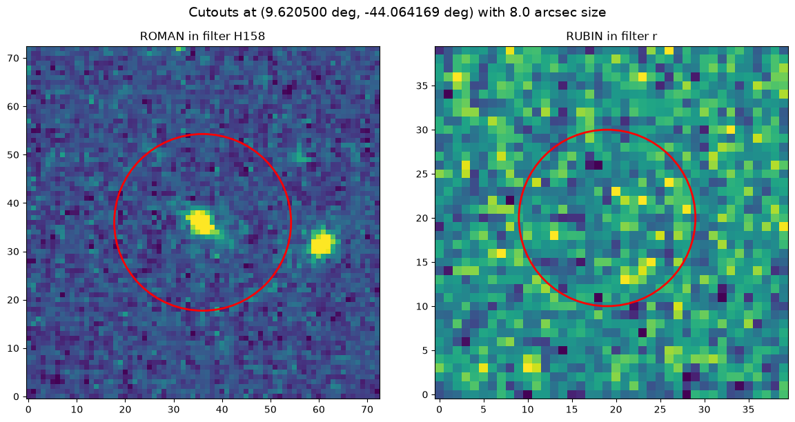

7. Use Firefly to visualize the OpenUniverse2024 catalogs¶

Let’s inspect the properties of sources in the Rubin image. For this we will use the input truth files present in S3 bucket.

OpenUniverse2024 includes the input truth files that were used to create the simulated images. These files are in Parquet and HDF5 format, and include information about the properties of galaxies, stars, and transients.

The catalogs are split by HEALPix sky region (nside=32, RING ordering) and the region index appears in each filename, so we can convert our sky position into that index with hpgeom rather than hunting through the directory listing. This is the same approach the Quickstart tutorial takes.

Each region comes as two separate catalogs: a point source catalog holding the stars, and a galaxy catalog. We load both below and overlay each on the image.

region = hpgeom.angle_to_pixel(32, coord.ra.deg, coord.dec.deg, lonlat=True, nest=False)
print(f"HEALPix region for our position: {region}")

HEALPix region for our position: 10307

# Catalog table of star properties (in parquet format)
pointsource_cat_path = f"{BUCKET_NAME}/{TRUTH_FILES_PATH}/pointsource_{region}.parquet"
pointsource_cat_path

# Catalog table of galaxy properties (in parquet format)
galaxy_cat_path = f"{BUCKET_NAME}/{TRUTH_FILES_PATH}/galaxy_{region}.parquet"
galaxy_cat_path

Use Firefly’s show_table to overlay the catalogs on the interactive image¶

Each catalog spans a whole HEALPix region, which is much larger than the image we are looking at, so we filter the table down to the sky area the Rubin image actually covers. (Note: you can remove filters through the table UI if you wish to see the entire data)

# Bound the catalogs by the footprint of the Rubin image we sent to Firefly.
footprint = image_rubin['wcs'].calc_footprint()
ra_bounds = (footprint[:, 0].min(), footprint[:, 0].max())
dec_bounds = (footprint[:, 1].min(), footprint[:, 1].max())

You can visualize catalogs interactively with Firefly using show_table. This capability can take many parameters. Here we will simply send our catalog to Firefly so that we can (a) see an interactive table; (b) see this table plotted over the image that we’ve already sent; and (c) use the GUI to quickly create exploratory plots. See if you can use the GUI to quickly determine approximately how many galaxies cover the Rubin image and what the redshift distribution of these galaxies is.

cat_filters = [
    f'("ra" >= {ra_bounds[0]} AND "ra" <= {ra_bounds[1]})', 
    f'("dec" >= {dec_bounds[0]} AND "dec" <= {dec_bounds[1]})'
]
cat_filters

fc.show_table(url=https_url(pointsource_cat_path),
              title='Stars Catalog',
              tbl_id='stars_cat',
              filters=" AND ".join(cat_filters))

WARNING: url is deprecated, use file_input parameter instead

gal_cat_tbl_id = 'galaxy_cat'

# may take ~1.25min, because galaxy catalog is a big file
fc.show_table(url=https_url(galaxy_cat_path),
              title='Galaxy Catalog',
              tbl_id=gal_cat_tbl_id,
              filters=" AND ".join(cat_filters))

WARNING: url is deprecated, use file_input parameter instead

For each row in the table you can notice a marker in the image. Selecting a row or marker changes the corresponding marker or row, respectively. You can click on “Details” tab in the UI to show properties of each source selected in image/table.

Use Firefly’s apply_table_filters to show only high-redshift galaxies¶

High redshift galaxies are the most interesting, so let’s filter the table we sent to Firefly to only include z>2.5 galaxies. Notice how the table display and image overlay change. Notice how the chart becomes a scatterplot from a heatmap because the sources reduce. You can remove this filter or add new ones through the GUI.

For filtering, we will use apply_table_filters method on the galaxy table we loaded above.

fc.apply_table_filters(tbl_id=gal_cat_tbl_id,
                       filters=" AND ".join(cat_filters+['"redshift" > 2.5']))

You can play with the filters directly from the UI as well. Try removing adding more filters in the tables and see how markers change.

Use Firefly’s show_fits_3color to create a 3 color image of the simulated Rubin images¶

# [R, G, B]
ROMAN_RGB_FILTERS = ['H158', 'J129', 'Y106']
RUBIN_RGB_FILTERS = ['r', 'g', 'u']

We already have a Rubin image with the catalog overlaid, let’s make a 3 color image to see colors of marked objects more clearly. For this we will use show_fits_3color method:

image_ff_id_rubin_3color = 'rubin-image-3color'
rubin_rgb_fpaths = get_rubin_image_fpaths(coord, RUBIN_RGB_FILTERS)
threeC = [
    dict(url=https_url(rubin_rgb_fpaths[filter_name]),
         Title="Rubin 3 color")
    for filter_name in RUBIN_RGB_FILTERS
]

fc.show_fits_3color(three_color_params=threeC,
                    plot_id=image_ff_id_rubin_3color)

Use Firefly’s interactivity to identify a region of interest¶

For example, we found a region of the sky that seems to have a high number of high redshift sources and we copy it from the image display:

# located and copied through UI
high_z_gal_coords = SkyCoord('0h38m28.62s -44d00m50.52s', frame='icrs')
high_z_gal_coords

# let's also mark it in our region layer, so that it's easy to pinpoint later
point_region = f'icrs;point {high_z_gal_coords.ra.value}d {high_z_gal_coords.dec.value}d # point=cross 15 text={{z>2.5 mock galaxies}}'
fc.add_region_data(region_data=point_region, region_layer_id=roman_regions_id,
                   plot_id=image_ff_id_rubin)

8. Plot 3-color Roman image containing your region of interest¶

Let’s inspect WCS of the Roman image first

image_roman['wcs']

Prepare Roman images for displaying in Firefly¶

The Roman exposures are gzipped on S3, so rather than hand Firefly a URL as we did for Rubin, we read each one in Python and pass it up as an in-memory FITS file.

def get_fits_stream(image_roman):
    """Write an image to an in-memory FITS file for handing to Firefly.

    Parameters
    ----------
    image_roman : dict
        Image dictionary with ``'data'`` and ``'wcs'`` keys, as returned by
        `get_roman_image`.

    Returns
    -------
    `~io.BytesIO`
        FITS file positioned at the start, ready to be read.
    """
    # Create a FITS PrimaryHDU object with the image data
    hdu = fits.PrimaryHDU(data=image_roman['data'], header=image_roman['wcs'].to_header())

    # Write the HDU to the in-memory stream (to save I/O time)
    fits_stream = BytesIO()
    hdu.writeto(fits_stream, overwrite=True)
    fits_stream.seek(0) # to bring reading pointer to the beginning of file

    return fits_stream

Then we read one exposure per RGB filter and turn each into a stream:

images_rgb = []
images_rgb_fits_stream = []

for filter_name in ROMAN_RGB_FILTERS:
    print(f'\nFILTER: {filter_name}')
    print('Retrieving Roman image...')
    image_roman = get_roman_image(high_z_gal_coords, filter_name)
    images_rgb.append(image_roman)

    print('Writing to fits stream...')
    images_rgb_fits_stream.append(get_fits_stream(image_roman))

FILTER: H158
Retrieving Roman image...

WARNING: FITSFixedWarning: 'datfix' made the change 'Changed DATE-OBS from '2028-05-19 13:41:34.224000' to '2028-05-19T13:41:34.224000''. [astropy.wcs.wcs]
WARNING: Some non-standard WCS keywords were excluded: A_ORDER, A_0_2, A_0_3, A_0_4, A_1_1, A_1_2, A_1_3, A_2_0, A_2_1, A_2_2, A_3_0, A_3_1, A_4_0, B_ORDER, B_0_2, B_0_3, B_0_4, B_1_1, B_1_2, B_1_3, B_2_0, B_2_1, B_2_2, B_3_0, B_3_1, B_4_0 Use the ``relax`` kwarg to control this. [astropy.wcs.wcs]

Writing to fits stream...

FILTER: J129
Retrieving Roman image...

WARNING: FITSFixedWarning: 'datfix' made the change 'Changed DATE-OBS from '2028-06-13 13:23:35.088000' to '2028-06-13T13:23:35.088000''. [astropy.wcs.wcs]

Writing to fits stream...

FILTER: Y106
Retrieving Roman image...

Writing to fits stream...

WARNING: FITSFixedWarning: 'datfix' made the change 'Changed DATE-OBS from '2028-11-05 14:42:46.310400' to '2028-11-05T14:42:46.310400''. [astropy.wcs.wcs]

Use Firefly’s show_fits_3color to create a 3 color image of Roman images¶

Now we upload each fits stream (in-memory fits file) to firefly using upload_fits_data() and prepare color params to pass to the show_fits_3color().

three_color_params = [
    {
        'file': fc.upload_fits_data(fits_stream),
        'Title': "Roman 3 color"
    } for fits_stream in images_rgb_fits_stream]

image_ff_id_roman_3color = 'roman-3color-high_z_gal'
fc.show_fits_3color(three_color_params=three_color_params,
                    plot_id=image_ff_id_roman_3color)

We can see a 3 color image of the Roman exposures containing the high-redshift galaxy sources. Try panning and zooming out; you can notice it covers a smaller patch of sky than the Rubin image.

Use Firefly’s pan/zoom/align methods to locate high redshift sources¶

Now, let’s pan & zoom to the region where we located high-redshift galaxy sources. Also align & lock all images being displayed by WCS. For these operations we use these 3 methods (click on them to see their documentation):

• set_pan

• set_zoom

• align_images

fc.set_pan(plot_id=image_ff_id_roman_3color, x=high_z_gal_coords.ra.deg, y=high_z_gal_coords.dec.deg, coord='j2000')
fc.set_zoom(plot_id=image_ff_id_roman_3color, factor=1)
fc.align_images(lock_match=True)

Use Firefly’s set_stretch method to change the stretch of the image display via Python¶

The image has a lot of noise that obscures our high redshift sources of interest. You can use the Firefly GUI to change the stretch of the image display. We identify that squared stretch from -2 to 10 sigma highlights the colors of our sources better. You can also use the Firefly client’s set_stretch to do this via Python. This is helpful for reproducibility and for scaling up to many images.

fc.set_stretch(plot_id=image_ff_id_roman_3color, stype='sigma', algorithm='squared', 
               band='ALL', lower_value=-2, upper_value=10)

About This Notebook¶

Updated: 2026-08-14

Contact: the IRSA Helpdesk with questions or reporting problems.